

This tutorial details Naive Bayes classifier algorithm, its principle, pros & cons, and provides an example using the Sklearn python Library.
This tutorial details Naive Bayes classifier algorithm, its principle, pros & cons, and provides an example using the Sklearn python Library.
Context
Let’s take the famous Titanic Disaster dataset. It gathers Titanic passenger personal information and whether or not they survived the shipwreck. Let’s try to make a prediction of survival using passenger ticket fare information.

Imagine you take a random sample of 500 passengers. In this sample, 30% of people survived. Among passenger who survived, the fare ticket mean is 100$. It falls to 50$ in the subset of people who did not survive. Now, let’s say you have a new passenger. You do not know if he survived or not, but you know he bought a 30$ ticket to cross the Atlantic. What is your prediction of survival for this passenger?
Principle
Ok, you probably answered that this passenger did not survive. Why? Because according to the information contained in the random subset of passengers, you assumed that chances of survival were low and that being poor reduced chances of survival. You put this passenger in the closest group of likelihood (the low fare ticket group). This is what the Naive Bayes classifier does.
How does it work?
The Naive Bayes classifier aggregates information using conditional probability with an assumption of independence among features. What does it mean? For example, it means we have to assume that the comfort of the room on the Titanic is independent of the fare ticket. This assumption is absolutely wrong, and it is why it is called Naive. It allows simplifying the calculation, even on very large datasets. Let’s find why.
The Naive Bayes classifier is based on finding functions describing the probability of belonging to a class given features. We write it P(Survival | f1,…, fn). We apply the Bayes law to simplify the calculation:

P(Survival) is easy to compute, and we do not need P( f1,…, fn) to build a classifier. It remains P(f1,…, fn | Survival) calculation. If we apply the conditional probability formula to simplify calculation again:

Each calculation of terms of the last line above requires a dataset where all conditions are available. To calculate the probability of obtaining f_n given the Survival, f_1, …, f_n-1 information, we need to have enough data with different values of f_n where condition {Survival, f_1, …, f_n-1} is verified. It requires a lot of data. We face the curse of dimensionality. Here is where the Naive Assumption will help. As feature are assumed independent, we can simplify calculation by considering that the condition {Survival, f_1, …, f_n-1} is equal to {Survival}:

Finally, to classify a new vector of features, we just have to choose the Survivalvalue (1 or 0) for which P(f_1, …, f_n|Survival) is the highest:

NB: One common mistake is to consider the probability outputs of the classifier as true. In fact, Naive Bayes is known as a bad estimator, so do not take those probability outputs too seriously.
Find the correct distribution function
One last step remains, to begin to implement a classifier. How to model the probability functions P(f_i| Survival)? There are three available models in the Sklearn python library:
- Gaussian: It assumes that continuous features follow a normal distribution.

- Multinomial: It is useful if your features are discrete.
- Bernoulli: The binomial model is useful if your features are binary.

Python Code
Here we implement a classic Gaussian Naive Bayes on the Titanic Disaster dataset. We will use Class of the room, Sex, Age, number of siblings/spouses, number of parents/children, passenger fare and port of embarkation information.
> Number of mislabeled points out of a total 357 points: 68, performance 80.95%The performance of our classifier is 80.95%.
Illustration with 1 feature
Let’s restrain the classification using the Fare information only. Here we compute the P(Survival = 1) and P(Survival = 0) probabilities:
> Survival prob = 39.50%, Not survival prob = 60.50%Then, according to the formula 3, we just need to find the probability distribution function P(fare| Survival = 0) and P(fare| Survival = 1). We choose the Gaussian Naive Bayes classifier. Thus we have to make the assumption that those distributions are Gaussian.

Then we have to find the mean and the standard deviation of the Fare datasets for different Survival values. We obtain the following results:
mean_fare_survived = 54.75
std_fare_survived = 66.91
mean_fare_not_survived = 24.61
std_fare_not_survived = 36.29
Let’s see the resulting distributions regarding survived and not_survived histograms:
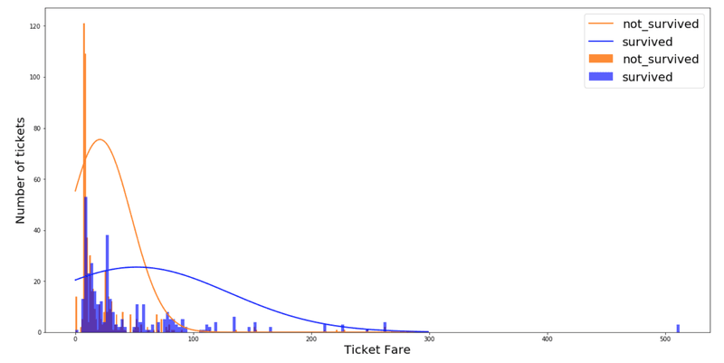
We notice that distributions are not nicely fitted to the dataset. Before implementing a model, it is better to verify if the distribution of features follows one of the three models detailed above. If continuous features do not have a normal distribution, we should use transformations or different methods to convert it in a normal distribution. Here we will consider that distributions are normal to simplify this illustration. We apply the Formula 1Bayes law and obtain this classifier:

If classifier(Fare) ≥ ~78 then P(fare| Survival = 1) ≥ P(fare| Survival = 0) and we classify this person as Survival. Else we classify as Not Survival. We obtain a 64.15% performance classifier.
If we train the Sklearn Gaussian Naive Bayes classifier on the same dataset. We obtain exactly the same results:
Number of mislabeled points out of a total 357 points: 128, performance 64.15%
Std Fare not_survived 36.29
Std Fare survived: 66.91
Mean Fare not_survived 24.61
Mean Fare survived: 54.75
Pro and cons of Naive Bayes Classifiers
Pros:
- Computationally fast
- Simple to implement
- Works well with small datasets
- Works well with high dimensions
- Perform well even if the Naive Assumption is not perfectly met. In many cases, the approximation is enough to build a good classifier.
Cons:
- Require to remove correlated features because they are voted twice in the model and it can lead to over inflating importance.
- If a categorical variable has a category in test data set which was not observed in training data set, then the model will assign a zero probability. It will not be able to make a prediction. This is often known as “Zero Frequency”. To solve this, we can use the smoothing technique. One of the simplest smoothing techniques is called. Sklearn applies Laplace smoothing by default when you train a Naive Bayes classifier.
Conclusion
Thank you for reading this article. I hope it helped you to understand what is Naive Bayes classification and why it is a good idea to use it.
Thanks to Antoine Toubhans, Flavian Hautbois, Adil Baaj, and Raphaël Meudec.
If you are looking for Machine Learning expert's, don't hesitate to contact us !