
Let me show you the magic of Mixed precision in Tensorflow, and you will be able to drastically reduce your transfer learning training resources in a few minutes!
I will explain what mixed precision is, what’s under the hood to make the magic happen, what material setup you need, and how to use it in TensorFlow.
If you’re a Pytorch user, make sure to stick around as most of this article will still be applicable to your projects.
Wait! What do we mean by “Mixed precision”?
Quoting the Tensorflow guide page for Mixed precision:
Mixed precision is the use of both 16-bit and 32-bit floating-point types in a model during training to make it run faster and use less memory. By keeping certain parts of the model in the 32-bit types for numeric stability, the model will have a lower step time and train equally as well in terms of the evaluation metrics such as accuracy. [...] Using this API can improve performance by more than 3 times on modern GPUs and 60% on TPUs.
Now that’s one big promise! But does it really translate to a real project?
Well yes! When trying Mixed precision on a Computer Vision project at Sicara, the results were as follows:
- Only 15 minutes to set up
- No significant change in metrics: the model had basically the same training trajectory and converged just as before
- GPU memory usage divided by 4
- -30% in total training time
In this case, no model hyperparameter was changed. However, reducing the GPU memory usage allows for bigger batches, which may reduce the training time even more dramatically.
What’s happening behind the scenes of Mixed precision?
Before diving into the Mixed precision paper, let’s see how a float is built.
How does one build a floating number?
In Computer Science, all numbers are encoded as bits, which represent powers of 2. This makes it simple to encode integers, but what about floating numbers? If you have already used the scientific notation of numbers, you know a good part of the answer!
Let us take the number -4,200,000,000. In scientific notation, you would write this number as -4.2 x (10^12). The first part is still a float because of scientific conventions, but you could rewrite using only integers as -42 x (10^11).
Now you can see there are 3 parts in this number: the sign (here a minus), the mantissa (42), and the exponent (11). You could write the exact same thing in base 2, which would give the number -1.95 x (2^31), giving a mantissa of 11110100101011011101010 and an exponent of 10011110 (see this converter). Your number can then be written as:
1 | 10011110 | 11110100101011011101010
where the first 1 encodes the negative sign, and the pipe signs separate the parts of the number but are not used in real cases.
Now the only difference between float number formats is the number of bits assigned to the mantissa and the exponent:
- float32 (aka single precision, on 32 bits) uses 8 bits for the exponent and 23 bits for the mantissa. Therefore, they can express numbers ranging from 1.18 x 10^(-38) to 3.4 x 10^38 (without taking the sign into account).
- float16 (aka half-precision, on 16 bits) uses 5 bits for the exponent and 10 bits for the mantissa, giving a range from 6.1 x 10^(-5) to 65504.
- You could also use bfloat16 (brain floating point) on TPUs. This format, invented by Google, keeps 8 bits for the exponent at the cost of using only 7 bits for the mantissa. There are 2 advantages to bfloat16: conversion from float32 is really easy as you just need to remove some bits from the mantissa, and you still keep the float32 exponent range.
Finally, when reading about float numbers, you might stumble into “FP16” or “FP32”, which are short for “float16” and “float32”.
How does mixed precision work?
The technique is called “mixed precision”, so as you might expect not all computations are made in half precision. Actually, training in FP16 precision only can lead to a reduction of performance [2].
Keeping the same model performance is made possible by 3 tweaks:
- A FP32 master copy of weights is used to update the weights because the updates might be too small compared to the weight itself. Using FP16 when the update is at least 2048 times smaller than the weight would lead to no update, and thus the loss of convergence.
- Also to avoid underflow, the loss value is scaled. Indeed, if the loss underflows in the FP16 scale, the convergence is lost. In Tensorflow, you can let the program find the optimal scale value by itself using the “dynamic” loss scale.
- Finally, some sensitive operations are still carried out in FP32 to avoid a reduction of model performance. These include vector dot products, sums across elements of a vector, or point-wise operations. From [2], the last 2 categories are memory-bandwidth limited and not sensitive to arithmetic speed, which means that these operations take the same time in FP32 and FP16 anyway.
For more details, refer to the mixed precision paper [2].
How to use mixed precision on your project
With great Mixed precision power comes an actually small setup! Let us look at what you need.
The material setup
This is the only hard part here!
To fully profit from the advantages of Mixed precision, you will need an NVIDIA GPU or TPU with a compute capability of at least 7.0. You can look up the compute capability of your device on this page. If you don’t know the name of your GPU, you can look it up by running the following command in your terminal:
nvidia-smi -LFrom the TensorFlow documentation page: “Examples of GPUs that will benefit most from mixed precision include RTX GPUs, the V100, and the A100”.
But what does “compute capability” mean exactly? The compute capability describes the general specifications and features of a compute device. Therefore, the higher the compute capability, the more recent features the compute device has.
In particular, compute capability 7.0 introduces mixed precision Tensor Cores for deep learning matrix arithmetic, which helps make mixed precision computations quicker.
What if I don’t have such compute device?
Even if you train on a CPU or an older GPU, you can still try out TensorFlow mixed precision. In my experience, when trying mixed precision on a GeForce GTX 1080 Ti (compute capability 6.1), I still observed the same reduction in GPU memory usage. However, the training time was still as long as without mixed precision.
Beware though if you try this API on CPU, as mixed precision is expected to run significantly slower on such devices.
Why is mixed precision slower on CPU?
To understand why some compute devices handle better mixed precision than others, you need to dig into how operations are handled depending on the float size, as in a paper from Nhut-Minh Ho and Weng-Fai Wong (see [1]).
From Ho, Nhut-Minh; Wong, Weng-Fai (September 1, 2017). "Exploiting half precision arithmetic in Nvidia GPUs" (PDF). Department of Computer Science, National University of Singapore. Retrieved January 30, 2023.
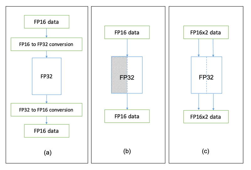
(a) In old GPU architectures and on most CPUs, FP16 numbers are treated as FP32, which requires casting to FP32 before computations and recast back to FP16 after. This makes more operations than for FP32 numbers, which explains why mixed precision is not preferable in such cases. This also means that if your GPU is really old, you might also experience slower training when using mixed precision.
(b) In slightly more recent GPUs (such as the GeForce GTX 1080 Ti I mentioned before), FP16 is natively supported. This means that there is no such time disadvantage for using this format.
(c) Finally, for GPUs with compute capability of at least 7.0, the FP32 Tensor core can be used to take two FP16 numbers at a time and execute the same computation on both of them. Such processing is called SIMD (Single Instruction, Multiple Data).
The code setup
Now for the easy part!
At the top of your training script, add these lines:
These lines make sure that, unless you specify otherwise, all TensorFlow layers defined after that will use the mixed precision policy, whether they are defined in your code or some other library.
Then, you have to make sure that the last layer of your model outputs at least FP32 precision numbers.
For example, if you are building a classifier for N classes, your last layer is probably defined as the following (before mixed precision):
With mixed precision, these lines become as follows:
Now for the final touch, you need to make sure that your loss is always in the range of FP16 numbers. This is because if you let your loss underflow or overflow, your model will no longer be able to train. For this, you can use the LossScaleOptimizer from mixed precision to wrap your optimizer, and it will do all this work for you. For instance, if you used the Adam optimizer, this can be done as the following:
The variable scaled_optimizer can then be used just like any optimizer you’re used to.
You’re now up and running! You can train your model with mixed precision and see the results by yourself.
As a use case, you can use mixed precision to fine-tune a Transformer model faster and with less resources.
And if you’re looking for even more optimization in Computer Vision, you might be interested in pruning your model.
Are you looking for Image Recognition Experts? Don't hesitate to contact us!
References
[1] Ho, Nhut-Minh; Wong, Weng-Fai (September 1, 2017). "Exploiting half precision arithmetic in Nvidia GPUs" (PDF). Department of Computer Science, National University of Singapore. Retrieved January 30, 2023.
[2] MICIKEVICIUS, Paulius, NARANG, Sharan, ALBEN, Jonah, et al. Mixed precision training. arXiv preprint arXiv:1710.03740, 2017.